14. Climate matrix

The climate matrix is based on the figures of the average temperature of the warmest month and of the average yearly temperature provided by the European meteorological stations. These data are adapted and simplified in such way that they are easy to use in the study of the climatological limitations of butterfly species and are also useful to predict shifts in distribution after expected changes in climate.
For that purpose the phrases ‘heat-sum’ and ‘climate window’ are introduced.

The relationship between climate characteristics and the occurrence of butterfly species is complex and to start such a study the use of easily obtainable figures with reference to climate can be helpful.
Basic data on climate are provided by the meteorological stations and the selected ones for use in a climate matrix are those of the average temperature of the warmest month (in Europe, July) and the yearly average temperature. The difference between both is the amplitude, a measure of the seasonal character. The greater the amplitude, the greater is the resemblance to a continental climate, with hot summers and cold winters. However, winter is not only the season having frosts but it is the season for snow-cover, a very important factor in the survival of insects hibernating in the herb-layer. A small amplitude indicates a maritime climate with cool summers and mild winters but also having a high unpredictability of the course of the seasons.
The data on the average temperature of the warmest month and of the yearly average permit a calculation of the amount of yearly warmth and the length of the summer season. The amount of warmth will be expressed here in degree-days over an average temperature of 10°C (see below) and the length of the growing season in days per year. For the calculation of both the construction of a climate diagram is necessary. The method of the calculation of the degree-days is developed after a goniometric exercise by Jan Bik (Bink & Bik 2009).

	The climate matrix illustrates the extent in different climates; it combines heat-sum and climate window. From a climate matrix it can be deduced how far to the north or to the south a species can survive, also the maximun altitude in mountainous regions at which a butterfly can survive. It demonstrates also how far a species can survive westwards in maritime and eastwards in continental climates. It is an interpretation based on published butterfly distribution records and data from meteorological stations. There are very narrow matrices that explain at a glance why some species are endangered and very broad matrices of species which seem to occur everywhere. The latter is not easy to interpret, the migration behaviour may be the main factor.
	The climate matrix of Lycaena phlaeas resembles that of the painted lady but has a very different environment. Photograph: Rosita Moenen ©.	Vanessa cardui is a migrant species having a climate matrix resembling the one of the small copper. Photograph: Rosita Moenen ©.
	The climate matrices of the small copper (Lycaena phlaeas) resembles that of the migrant species, of tropical origin, the painted lady (Vanessa cardui); however the two species differ very much in their environments.

Threshold temperature
To obtain a heat threshold of biological meaning only the average temperature over 10°C will be considered. (This threshold temperature was chosen by Walter & Lieth 1967, Walter 1990.) This temperature threshold is an arbitrary value and from the biological point of view it is roughly related to the period that broadleaved trees are growing. In spring when the average temperature reach 10°C the buds will burst and in autumn when the average temperature drops below 10°C, the leaves will start to fall.

Climate diagrams
IThe meteorological stations present yearly data about average monthly temperatures. The data of a particular region or spot can be arranged in a sinus-like figure, the ‘climate diagram’. When this figure is considered as a sine curve the data of average temperature of the warmest month and the yearly average can be seen. The average temperature of the warmest month is at the top of the curve and the difference between it and the average yearly temperature is the value of the amplitude.
The 10°C line in the diagram, an arbitrary threshold temperature of biological activity, intersects the sine curve at two points and a perpendicular line drawn from these points towards the base line will mark the intersection. The base line is divided in 364 days and the period the average temperature will be over 10°C can be read as the period of the growing season, called the ‘climate window’ and expressed in days per year.
The area of the curve between the intersection points on the 10°C threshold line and the top of the curve can be seen as a measure of warmth and named the ‘heat-sum’ and expressed in ‘degree-days’. In this study each degree Celsius of temperature above the threshold temperature of 10°C. This area can be calculated after the method described in Bink & Bik (2009).
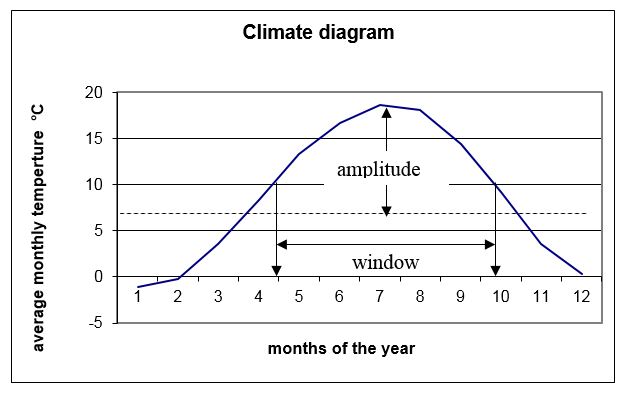
In figure 14-1 the curve represents a climate with an average July-temperature of 18°C (the top of the curve) and the average yearly temperature of 6°C (the horizontal dotted line). The amplitude is 12 (18 minus 6) and this indicates that it represents a continental climate. The calculated heat-sum is 728°d and the climate window 143 days. In this type of climate the growing season is little more than 20 weeks.

Figure 14-1. Scheme of a climate diagram

Climate matrix
A climate matrix can be composed with July-temperature along the y-axis and the amplitude along the x-axis. The heat-sum and length of the climate window has been calculated and filled in for every combination. In appendix 5, 6 these matrices are recorded in detail and appendix 7 presents the rounded off figures.

Examples
Data from the Dutch meteorological institute K.N.M.I. at the Bilt over the period 1976-2006:

Yearly average 10.0°C
July average 17.7°C
amplitude 17.7 – 10.0 = 7.7
Calculated heat-sum 899 °d
Calculated climate window 184 days

In a climate diagram the point at which the average July temperature occurs is at day 197 and the climate window will begin at day 105 (15th of April) and will end at day 289 (15th of October).
In the case of another threshold temperature instead of 10°C being chosen, for example 7°C, a temperature that better represents the growing activity in a habitat of herbs and grasses, the climate window will be 232 days and starts on 22nd of March and ends on 9th of November.
In the same way the climate windows and heat-sums of the capitals of the Benelux can be calculated, see table 14-1 for results.

Table 14-1. Climate windows and heat-sums of the capitals in the Benelux.

The heat-sum of 900 °d occurs under different combinations of average July-temperature, amplitude and climate window. In Europe the heat-sum of 900 °d can be measured from Scilly Islands up to Siberia (see table 14-2).

Table 14-2. Heat-sum of 900 °d for various localities in Europe.

The amplitude 8 is in between maritime and continental climates and occurs in Europe in a zone from north Norway to the east side of southern Spain. In this zone of amplitude 8 the July-temperature, heat-sum and climate window can occur in various different values (see examples in table 14-3).

Table 14-3. Amplitude 8 with various values of temperature, heat-sum and climate window.

Climate matrix on a European scale
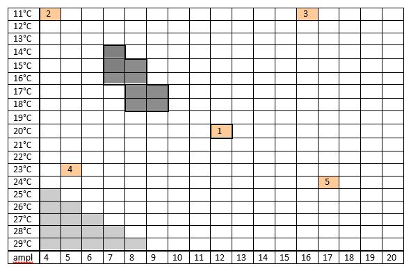
The values of the parameters of the matrix are chosen for the July temperature from 11°C, the subarctic region in the high north, and up to 29°C in the tropical region. The amplitude ranges from 4, an extreme maritime climate, up to 20, the extreme continental climate in Siberia.
The central point of the matrix corresponds with 20°C July temperature and amplitude 12. This is typically for a continental climate with normal summer warmth as in Kiev (20.0 °C & 12.9) and Lviv (20.0 °C & 11.6) in the Ukraine. This cell is numbered as one in figure 14-2. In this figure cell 2 concerns a cold maritime climate as at Tórshavn, Faroe Islands (10.8°C & 4.4), cell 3 the Russian tundra in Pustogersk (11.4°C & 16,1), cell 4 the subtropics at Lagos, Portugal (23.1°C & 5.4) and cell 5 the Russian steppe at Volgograd (23.6°C & 17.2).
The climate in the Benelux varies from cool mountainous on the Hautes Fagnes (14°C & 7), cool maritime on the West Frisian Islands (16°C & 7) and to rather warm sub-continental in the south of Luxemburg and Wallonia (18°C & 9). A cluster of 9 cells are marked in the matrix to illustrate the variety of climate that occurs in the Benelux. This cluster is illustrated in the appendix ‘matrix per species’ and clarifies at a glance how far the species is restricted inside this area.

Figure 14-2. Position of the Benelux in the European climate matrix indicated by the cluster of dark cells.
Other cells: 1 Ukraine, 2 Faroe Islands, 3 Russian tundra, 4 subtropical Portugal, 5 Russian steppe.
The shaded corner of matrix 25 - 4 / 29 - 8 represents a tropical climate not occurring in Europe.

A point of note: a heat-sum of a locality in the high north is not the same as an equal heat-sum in the Alps. In boreal regions daylight is very long in summer, the sun is low in the sky and its radiation is mild, whereas in the Alps the days in summertime are much shorter but the solar radiation much stronger. In the latter habitats the difference between day and night temperatures is great and there is often frost during the night. This factor is responsible for the differences in the species composition of both flora and fauna in boreal and alpine habitats.

Basic character of the matrix
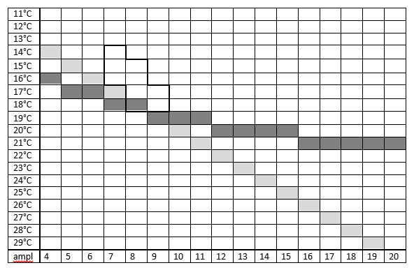
The two parameters of the matrix interact. The average temperature of the warmest month and the amplitude produce figures of the combination of the heat-sum and the climate window which are unique. How this works can be demonstrated in figure 14-3. The climate window of 26 weeks produce a straight line, from 14°C & 4 to 29°C & 19 (shown lightly shaded). However, the heat-sum of 900° a J-shaped line, from 16°C & 4 to 21°C & 20 (shown darkly shaded). In the cells 18°C & 8 and 19°C & 9 the climate window line and heat-sum line share the same cells.
This interaction of temperature and amplitude is remarkable. Every combination of these parameters produces a unique result. These idiographic details can be read from the matrices of heat-sums and from the climate windows. Only in the Benelux, at 18°C & 8 and 19°C & 9, the cells share the same parameters. See figure 14-3.

Figure 14-3. Unexpected characteristics of the climate window and heat-sum.
Diagonally the line of figures of the climate window, after a J-shaped line the figures of heat-sums.

Application
The required heat-sum of a species at the northern limit of its distribution area is considered as a property of the species. The value can be read from the matrix of the heat-sums (see table 14-3).
The zone of amplitude 8 in Europe reaches from Tromsö in Norway where the average July-temperature is only 12°C and reaches Murcia in Spain where the July-temperature is 26°C.
The heat-sum at Tromsö is about 100°d, those at Murcia 2900°d.

The most northern site where a species occurs in the zone of amplitude 8 is considered to be the site where it is just warm enough for the required heat-sum. The local average temperature of July is derived from the data of the nearby meteorological station in the lowland.
Where the northern boundary of a species distribution area meets the zone of amplitude 8, the local heat-sum is regarded as the required value for that species. In the same way, the southern boundary is the limit of the maximal tolerated heat-sum.

Example
At 24°C July-temperature and amplitude 8 the heat-sum is 2270°d (see the matrix in appendix 5). Going to the east the amplitude will increase, and at amplitude 17 the corresponding heat-sum is only 1453°d.
Going from Rome to Volgograd there is a strong decline in heat-sum, though in mid-summer it is often very hot in Volgograd. This explains that in the Mediterranean climate of Rome many species are double brooded, whereas in the continental climate of Volgograd these butterflies may produce only a single brood in spite of the hot summer.
There is little known about the occurrence of the species on localities in an extreme continental climate (29°C/20), where the heat-sum is 2129°d, nearly the same as in Mediterranean localities at 24°C/8, where the heat-sum is 2270°d. In the matrices the heat-sum values observed above amplitude 8 are too uncertain to consider and are therefore only vaguely indicated.

Appendices
There are three matrices concerning the values about the climate data. The calculated data are recorded in detail in the matrix ‘Heat-sum’ (Appendix 3) and in the matrix ‘Climate-window’ (Appendix 4). Both matrices are combined and simplified in the matrix ‘Heat-sum & Climate-window’ (Appendix 5) where the values are presented per cell. The heat-sum figures are simplified and the climate-windows reduced to weeks per year.
The figures on climate should be applicable for the biological ones. The required time to complete the lifecycle is also given in weeks and thus easy to compare with climate-window figures. The figures of the combined climate-window and heat-sum matrix are used in the species accounts.

References
Asher et al. (2001), Barkman & Stoutjesdijk (1987), Bink (1992), Bink & Bik (2009), Bos et al. (2006), Boszko (1997), Bryant, Bale & Thomas (1998), Bryant, Thomas & Bale (2002), Ebert & Rennwald (1991a, b), Fichefet et al. 2008), Cuvelier et al. (2007), Gonseth (1987), Henriksen & Kreutzer (1982), Hasselbarth, Van Oorschot & Wagner (1995), Korshunov & Gorbunov (1995), Kudrna et al. (2011), Lafranchis (2000), Lafranchis (2015), Meteorological Office (1958), Settele et al. (2009), Stolze (1994), Svindov (1982), Thust, Kun & Rommel (2006), Walter & Lieth (1967), Walter (1990)

Appendix 3. Matrix of heat-sums
Appendix 4. Matrix of climate windows
Appendix 5. Matrix of rounded off figures of heat-sum and climate window

Contact: Sylvain Cuvelier